Introduction

A [geographical] map is a representation of a geographical space. It highlights the extent of this space, its relative location in relation to neighboring spaces, as well as the location of the elements it contains. Maps are also used to represent geographical phenomena, that is to say phenomena whose spatial configuration produces meaning.

library(sf)      # for the map
library(dplyr)   # for data manipulation (and the pile : %>%)
library(ggplot2) # for plottingNot run)

Loading the shapefile

We are going to use the shapefile of the Democratic Republic of Congo, which can be found online in the WFPGeoNode website. In most cases, the files downloaded will be zipped. After unzipping, store all the files in the same folder.

In our case, our shape files are stored in a folder named shp and contains 6 files. The file we will load ends with .shp.

setwd("shp/") 
dir()
[1] "cod_admbnda_adm2_rgc_20170711.cst" "cod_admbnda_adm2_rgc_20170711.dbf"
[3] "cod_admbnda_adm2_rgc_20170711.prj" "cod_admbnda_adm2_rgc_20170711.shp"
[5] "cod_admbnda_adm2_rgc_20170711.shx" "wfsrequest.txt"                   

The following command reads the shape file and stores it in drc_shape object

drc_shape <- st_read("shp/cod_admbnda_adm2_rgc_20170711.shp")
Reading layer `cod_admbnda_adm2_rgc_20170711' from data source 
  `C:\Users\user\Desktop\bervelin-lumesa.github.io\content\blog\2022-02-25-r-mapping-data-in-r\shp\cod_admbnda_adm2_rgc_20170711.shp' 
  using driver `ESRI Shapefile'
Simple feature collection with 240 features and 14 fields
Geometry type: POLYGON
Dimension:     XY
Bounding box:  xmin: 12.20566 ymin: -13.456 xmax: 31.30522 ymax: 5.386098
Geodetic CRS:  WGS 84

Let’s explore a bit the content of drc_shape with some basic R functions.

class(drc_shape)
[1] "sf"         "data.frame"

We can see that the object drc_shape has two classes, sf and data.frame. It means that it can be manipulated like standard dataframes.

str() function indicates that our data.frame contains 240 observations and 15 varibleas. At the end, we have geometry which contains geographical informations.

str(drc_shape)
Classes 'sf' and 'data.frame':  240 obs. of  15 variables:
 $ Shape_Leng: num  2.34 5.53 0.13 7.25 5.23 ...
 $ Shape_Area: num  0.15237 0.50781 0.00124 1.11504 0.74832 ...
 $ ADM2_FR   : chr  "Tshilenge" "Popokabaka" "Bulungu" "Isangi" ...
 $ ADM2_PCODE: chr  "CD8202" "CD3108" "CD3205" "CD5105" ...
 $ ADM2_REF  : chr  "Tshilenge" "Popokabaka" "Bulungu" "Isangi" ...
 $ ADM2ALT1FR: chr  "<Null>" "<Null>" NA "<Null>" ...
 $ ADM2ALT2FR: chr  NA NA NA NA ...
 $ ADM1_FR   : chr  "Kasaï-Oriental" "Kwango" "Kwilu" "Tshopo" ...
 $ ADM1_PCODE: chr  "CD82" "CD31" "CD32" "CD51" ...
 $ ADM0_FR   : chr  "République Démocratique du Congo" "République Démocratique du Congo" "République Démocratique du Congo" "République Démocratique du Congo" ...
 $ ADM0_PCODE: chr  "CD" "CD" "CD" "CD" ...
 $ date      : Date, format: "2017-05-29" "2017-05-29" ...
 $ validOn   : Date, format: "2017-07-10" "2017-07-10" ...
 $ ValidTo   : Date, format: NA NA ...
 $ geometry  :sfc_POLYGON of length 240; first list element: List of 2
  ..$ : num [1:422, 1:2] 23.7 23.7 23.7 23.7 23.7 ...
  ..$ : num [1:17, 1:2] 23.6 23.6 23.6 23.6 23.6 ...
  ..- attr(*, "class")= chr [1:3] "XY" "POLYGON" "sfg"
 - attr(*, "sf_column")= chr "geometry"
 - attr(*, "agr")= Factor w/ 3 levels "constant","aggregate",..: NA NA NA NA NA NA NA NA NA NA ...
  ..- attr(*, "names")= chr [1:14] "Shape_Leng" "Shape_Area" "ADM2_FR" "ADM2_PCODE" ...

unique() with a variable name as an argument gives us names of the 26 provinces of the country (DRC).

unique(drc_shape$ADM1_FR)
 [1] "Kasaï-Oriental" "Kwango"         "Kwilu"          "Tshopo"        
 [5] "Ituri"          "Kongo-Central"  "Bas-Uele"       "Haut-Uele"     
 [9] "Maï-Ndombe"     "Equateur"       "Nord-Kivu"      "Maniema"       
[13] "Lualaba"        "Haut-Lomami"    "Tanganyika"     "Sud-Ubangi"    
[17] "Nord-Ubangi"    "Mongala"        "Tshuapa"        "Sankuru"       
[21] "Sud-Kivu"       "Haut-Katanga"   "Lomami"         "Kinshasa"      
[25] "Kasaï-Central"  "Kasaï"         

In this article, we are going to work with the Kwango province. So we create a subset of the main dataset and store it in an objet called kwango_shape.

kwango_shape <- drc_shape %>%
  filter(ADM1_FR == "Kwango")

The first map

Let’s create the first map with ggplot2 and geom_sf() from sf package. Note that color argument with “blue” as value is used inside geom_sf() to change the color of border lines and fill for the color of the map.

ggplot(data = kwango_shape) + 
  geom_sf(color = "blue", fill = "white") + 
  ggtitle(label = "Kwango province map") + 
  theme_void()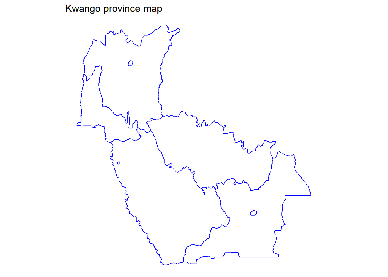

Mapping points with longitude and latitude

Suppose that we want to plot gps coordinates on the our previous map to see where the survey took place. For that, we need two columns : longitude and latitude. In the following code, we create a sample dataset (survey_df) containing four variables : longitude, latitude, status, ADM1_FR and num.

# creating a random dataset
set.seed(14) # to make the dataset reproducible
survey_df <- data.frame(longitude = rnorm(20, mean = 18, sd = 0.7),
                        latitude  = rnorm(20, mean = -7, sd = 0.5),
                        status    = sample(c("O", "N"), 20, replace = T),
                        region    = sample(kwango_shape$ADM2_FR, 20, replace = T),
                        num       = rnorm(20, mean = 200, sd = 20)
                     )

Let’s map now…

ggplot(data = kwango_shape) + 
  geom_sf(color = "blue", fill = "white") + 
  geom_point(data= survey_df, aes(x = longitude, y = latitude, color = status), size = 3) + 
  ggtitle(label = "Kwango province map with points") + 
  theme_void()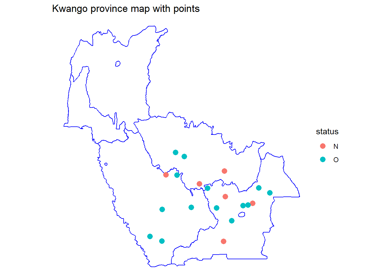

Thematic map

The following code allows to join two datasets kwango_shape and survey_sum with the dplyr’s function left_join(). The by argument allows to specify key columns for joining two tables.

Note that we first calculate the mean value of our numeric variable grouped by region.

survey_sum <- survey_df %>%
  group_by(region) %>%
  summarise(num = mean(num))

all_df <- kwango_shape %>%
  left_join(survey_sum, by = c("ADM2_FR" = "region"))

To create a thematic map, in the geom_sf() function, inside aes(), we use the fill argument giving it the name of the variable to illustrate.

ggplot() + 
  geom_sf(data =all_df, aes(fill = num), color = "white") + 
  ggtitle(label = "Kwango province Thematic map") + 
#  scale_fill_gradient2("Variable to illustrate", low = "white", high = "blue") + 
  scale_fill_viridis_c("Variable to illustrate") + 
  theme_void()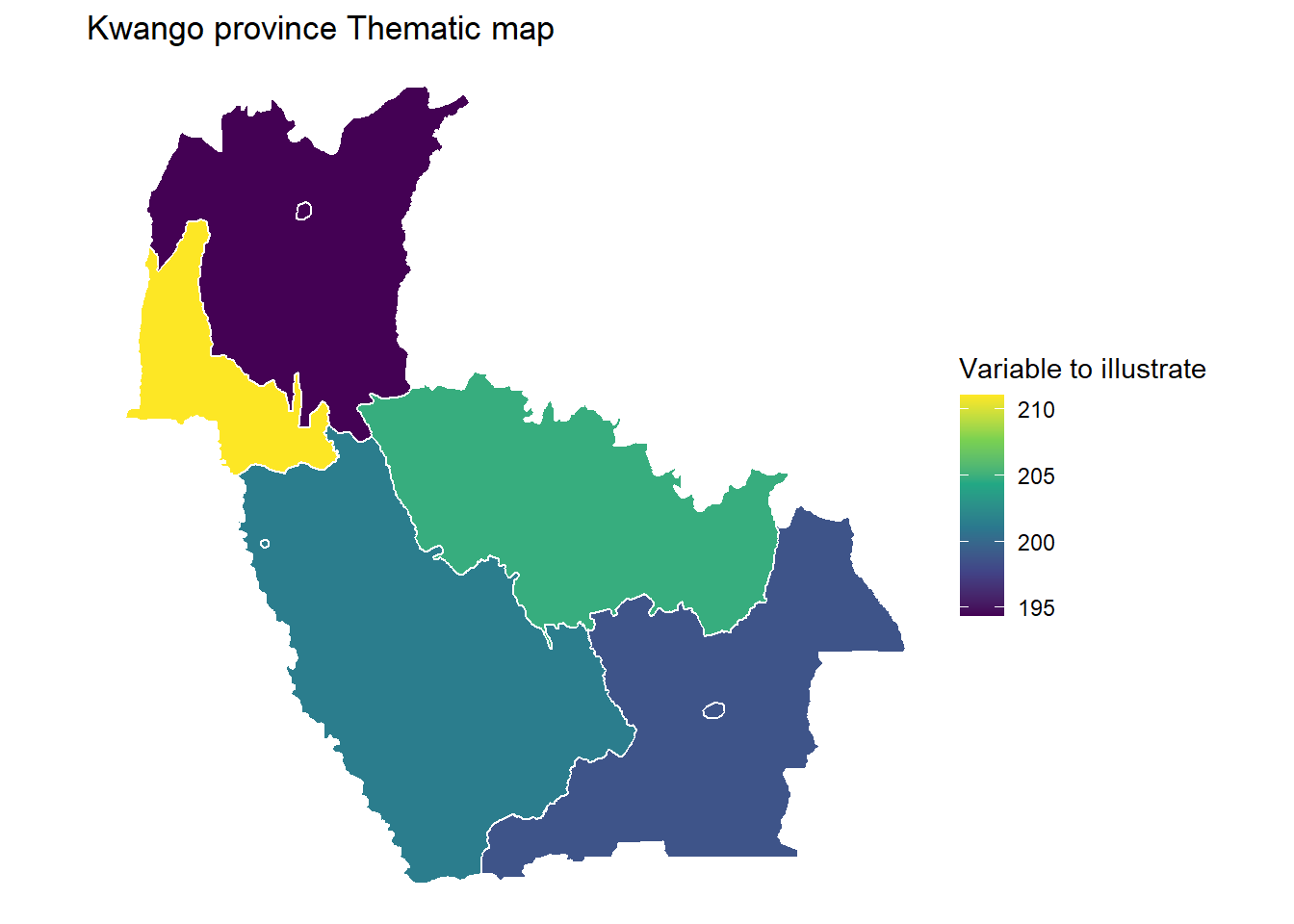

We know that Kwango, Kwilu and Maï-Ndombe were parts of The old Bandundu province before decentralization. Let’s build a map containing all the three provinces.

ggplot() + 
  geom_sf(data = drc_shape %>% filter(ADM1_FR %in% c("Kwango", "Kwilu", "Maï-Ndombe")), fill = "white") + 
  geom_sf(data =all_df, aes(fill = num), color = "white") + 
  ggtitle(label = "Old Bandundu province") + 
#  scale_fill_gradient2("Variable to illustrate", low = "white", high = "blue") + 
  scale_fill_viridis_c("Variable to illustrate") + 
  theme_void()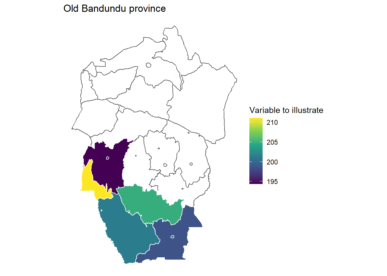

Finishing…

Currently R contains tens of packages to work with geographic data. What was shown here is less than 0.25% of what can be done with geographic data in R. For further reading, check the links below

• Geocomputation with R
• ggplot2: Elegant Graphics for Data Analysis
• Create a data frame of map data

All the code of this article and others can be downloaded in Github.

Was this article helpful ? Don’t forget to share it !

TO KUTANI MBALA YA SIMA :)