In this article, we describe what Exploratory Data Analysis is and see how to perform it with R.
Introduction to R and Rstudio
R is an open-source software environment for statistical computing and graphics. R compiles and runs on Windows, Mac OS X, and numerous UNIX platforms (such as Linux). The R software project was first started by Robert Gentleman and Ross Ihaka. As of 2022, there were more than 3,000 such packages hosted on CRAN. R can be installed from the CRAN website
RStudio is an integrated development environment (IDE) that adds modern features like syntax highlighting to R. The strength of RStudio is that it brings all the features that you need together in one place.
Introduction to EDA
Exploratory data analysis is the process of exploring your data, and it typically includes examining the structure and components of your dataset, the distributions of individual variables, and the relationships between two or more variables. Visualization is the most heavily relied upon tool for exploratory data analysis to get a deep understanding of your data.
Exploratory analysis helps us ask better questions, but it does not answer questions. More specifically, we explore data in order to:
- Understand data properties such as nonlinear relationships, the existence of missing values, the existence of outliers, etc.
- Find patterns in data such as associations, group differences, confounders, etc.
- Suggest modeling strategies such as linear vs. nonlinear models, transformation
In the Tidyverse Skills for Data Science in R, authors summarized the general principales of EDA as follows :
- Look for missing values
- Look for outlier values
- Use plots to explore relationships
- Use tables to explore relationships
- If necessary, transform variables
A detective investigating a crime needs both tools and understanding. If he has no fingerprint powder, he will fail to find fingerprints on most surfaces. If he does not understand where the criminal is likely to have put his fingers, he will not look in the right places. Equally, the analyst of data needs both tools and understanding. - John W. Tukey
As stated in the quote above, doing Exploratory Data analysis requires to have tools and understanding. In our case, the R language with all its useful functions can be considered as our tool and the domain knowledge as our understanding.
Practice
Data
Data used in this post are from the questionr package. hdv2003 is a sample from 2000 people and 20 variables taken from the Histoire de Vie survey, produced in France in 2003 by INSEE. questionr package can be installed as other packages by typing : install.packages("questionr") and load to your RStudio session with the following command : library(questionr). Finally, data(hdv2003) allows to access data.
Apart from the questionr package where our data come from, we will also use some functions from the tidyverse package for data minipulation and graphics and the naniar package for missing data visualization. So you need to do the same work as with questionr package, except the last command.
EDA with R
First of all, we need to load packages we’ll work with and our data.
Note that our data.frame is transformed to a tibble with as_tibble() for convenient display of our data.
# libraries
library(tidyverse)
library(questionr)
library(naniar)

# data
data(hdv2003)

hdv2003 <- as_tibble(hdv2003)
The following command allows us to know the dimension of our dataset.
dim(hdv2003)
[1] 2000   20
Our dataset contains 2000 observations and 20 variables.
names() or colnames() returns the variable names of the dataset.
names(hdv2003)
 [1] "id"            "age"           "sexe"          "nivetud"
 [5] "poids"         "occup"         "qualif"        "freres.soeurs"
 [9] "clso"          "relig"         "trav.imp"      "trav.satisf"
[13] "hard.rock"     "lecture.bd"    "peche.chasse"  "cuisine"
[17] "bricol"        "cinema"        "sport"         "heures.tv"
Now, we would like to see the structure of our dataset. The str() gives the data type of variables and a look at some rows.
str(hdv2003)
tibble [2,000 x 20] (S3: tbl_df/tbl/data.frame)
 $ id           : int [1:2000] 1 2 3 4 5 6 7 8 9 10 ...
 $ age          : int [1:2000] 28 23 59 34 71 35 60 47 20 28 ...
 $ sexe         : Factor w/ 2 levels "Homme","Femme": 2 2 1 1 2 2 2 1 2 1 ...
 $ nivetud      : Factor w/ 8 levels "N'a jamais fait d'etudes",..: 8 NA 3 8 3 6 3 6 NA 7 ...
 $ poids        : num [1:2000] 2634 9738 3994 5732 4329 ...
 $ occup        : Factor w/ 7 levels "Exerce une profession",..: 1 3 1 1 4 1 6 1 3 1 ...
 $ qualif       : Factor w/ 7 levels "Ouvrier specialise",..: 6 NA 3 3 6 6 2 2 NA 7 ...
 $ freres.soeurs: int [1:2000] 8 2 2 1 0 5 1 5 4 2 ...
 $ clso         : Factor w/ 3 levels "Oui","Non","Ne sait pas": 1 1 2 2 1 2 1 2 1 2 ...
 $ relig        : Factor w/ 6 levels "Pratiquant regulier",..: 4 4 4 3 1 4 3 4 3 2 ...
 $ trav.imp     : Factor w/ 4 levels "Le plus important",..: 4 NA 2 3 NA 1 NA 4 NA 3 ...
 $ trav.satisf  : Factor w/ 3 levels "Satisfaction",..: 2 NA 3 1 NA 3 NA 2 NA 1 ...
 $ hard.rock    : Factor w/ 2 levels "Non","Oui": 1 1 1 1 1 1 1 1 1 1 ...
 $ lecture.bd   : Factor w/ 2 levels "Non","Oui": 1 1 1 1 1 1 1 1 1 1 ...
 $ peche.chasse : Factor w/ 2 levels "Non","Oui": 1 1 1 1 1 1 2 2 1 1 ...
 $ cuisine      : Factor w/ 2 levels "Non","Oui": 2 1 1 2 1 1 2 2 1 1 ...
 $ bricol       : Factor w/ 2 levels "Non","Oui": 1 1 1 2 1 1 1 2 1 1 ...
 $ cinema       : Factor w/ 2 levels "Non","Oui": 1 2 1 2 1 2 1 1 2 2 ...
 $ sport        : Factor w/ 2 levels "Non","Oui": 1 2 2 2 1 2 1 1 1 2 ...
 $ heures.tv    : num [1:2000] 0 1 0 2 3 2 2.9 1 2 2 ...
We can see that some variables are numeric, integer, while others are factors (lables with numeric values associated). If you think that a certain variable has the wrong type, functions like as.numeric(), as.factor(), as.Date() can be used to fix.
The following output uses head() and tail() to print the first and the last six rows of our dataset.
head(hdv2003)
# A tibble: 6 x 20
     id   age sexe  nivetud         poids occup qualif freres.soeurs clso  relig
  <int> <int> <fct> <fct>           <dbl> <fct> <fct>          <int> <fct> <fct>
1     1    28 Femme Enseignement s~ 2634. Exer~ Emplo~             8 Oui   Ni c~
2     2    23 Femme <NA>            9738. Etud~ <NA>               2 Oui   Ni c~
3     3    59 Homme Derniere annee~ 3994. Exer~ Techn~             2 Non   Ni c~
4     4    34 Homme Enseignement s~ 5732. Exer~ Techn~             1 Non   Appa~
5     5    71 Femme Derniere annee~ 4329. Retr~ Emplo~             0 Oui   Prat~
6     6    35 Femme Enseignement t~ 8675. Exer~ Emplo~             5 Non   Ni c~
# ... with 10 more variables: trav.imp <fct>, trav.satisf <fct>,
#   hard.rock <fct>, lecture.bd <fct>, peche.chasse <fct>, cuisine <fct>,
#   bricol <fct>, cinema <fct>, sport <fct>, heures.tv <dbl>

tail(hdv2003)
# A tibble: 6 x 20
     id   age sexe  nivetud         poids occup qualif freres.soeurs clso  relig
  <int> <int> <fct> <fct>           <dbl> <fct> <fct>          <int> <fct> <fct>
1  1995    46 Femme Enseignement ~  8408. Au f~ Autre              0 Non   Appa~
2  1996    45 Homme Enseignement ~  8092. Exer~ Techn~             3 Non   Ni c~
3  1997    46 Homme Enseignement ~   956. Exer~ Ouvri~             4 Oui   Prat~
4  1998    24 Homme Enseignement ~  5320. Exer~ Techn~             1 Oui   Rejet
5  1999    24 Femme Enseignement ~ 13741. Exer~ Emplo~             2 Non   Appa~
6  2000    66 Femme Enseignement ~  7710. Au f~ Emplo~             3 Non   Appa~
# ... with 10 more variables: trav.imp <fct>, trav.satisf <fct>,
#   hard.rock <fct>, lecture.bd <fct>, peche.chasse <fct>, cuisine <fct>,
#   bricol <fct>, cinema <fct>, sport <fct>, heures.tv <dbl>
To get a statistical summary of our data, we use the summary() function which gives the minimum, first and third quantiles, mean, median and the maximum values of all numeric variables. For categorical variables (factor), it counts the number of observations within each category.
summary(hdv2003)
       id              age           sexe
 Min.   :   1.0   Min.   :18.00   Homme: 899
 1st Qu.: 500.8   1st Qu.:35.00   Femme:1101
 Median :1000.5   Median :48.00
 Mean   :1000.5   Mean   :48.16
 3rd Qu.:1500.2   3rd Qu.:60.00
 Max.   :2000.0   Max.   :97.00

                                                 nivetud        poids
 Enseignement technique ou professionnel court       :463   Min.   :   78.08
 Enseignement superieur y compris technique superieur:441   1st Qu.: 2221.82
 Derniere annee d'etudes primaires                   :341   Median : 4631.19
 1er cycle                                           :204   Mean   : 5535.61
 2eme cycle                                          :183   3rd Qu.: 7626.53
 (Other)                                             :256   Max.   :31092.14
 NA's                                                :112
                   occup                           qualif    freres.soeurs
 Exerce une profession:1049   Employe                 :594   Min.   : 0.000
 Chomeur              : 134   Ouvrier qualifie        :292   1st Qu.: 1.000
 Etudiant, eleve      :  94   Cadre                   :260   Median : 2.000
 Retraite             : 392   Ouvrier specialise      :203   Mean   : 3.283
 Retire des affaires  :  77   Profession intermediaire:160   3rd Qu.: 5.000
 Au foyer             : 171   (Other)                 :144   Max.   :22.000
 Autre inactif        :  83   NA's                    :347
          clso                              relig
 Oui        : 936   Pratiquant regulier        :266
 Non        :1037   Pratiquant occasionnel     :442
 Ne sait pas:  27   Appartenance sans pratique :760
                    Ni croyance ni appartenance:399
                    Rejet                      : 93
                    NSP ou NVPR                : 40

                         trav.imp           trav.satisf  hard.rock  lecture.bd
 Le plus important           : 29   Satisfaction  :480   Non:1986   Non:1953
 Aussi important que le reste:259   Insatisfaction:117   Oui:  14   Oui:  47
 Moins important que le reste:708   Equilibre     :451
 Peu important               : 52   NA's          :952
 NA's                        :952


 peche.chasse cuisine    bricol     cinema     sport        heures.tv
 Non:1776     Non:1119   Non:1147   Non:1174   Non:1277   Min.   : 0.000
 Oui: 224     Oui: 881   Oui: 853   Oui: 826   Oui: 723   1st Qu.: 1.000
                                                          Median : 2.000
                                                          Mean   : 2.247
                                                          3rd Qu.: 3.000
                                                          Max.   :12.000
                                                          NA's   :5
You may also use glimse() function from the skimr() package like this skimr::skim(hdv2003)
We see for instance that the mean age is 48.16, with minimum of 18 and 97 as maximum. Our data contains more women (1101) than men (899).
summary() can also be used to describe a single variable, while table() or freq() (from questionr) is used for a categorical variable.
summary(hdv2003$age)
   Min. 1st Qu.  Median    Mean 3rd Qu.    Max.
  18.00   35.00   48.00   48.16   60.00   97.00
freq(hdv2003$relig)
n % val%
Pratiquant regulier 266 13.3 13.3
Pratiquant occasionnel 442 22.1 22.1
Appartenance sans pratique 760 38.0 38.0
Ni croyance ni appartenance 399 20.0 20.0
Rejet 93 4.7 4.7
NSP ou NVPR 40 2.0 2.0From the output of the first summary function call, we notice that some variables have many missing data. For instance, qualif has 347 missings whereas trav.satisf and trav.imp have 952 missing values.
We can use the vis_miss() function from the naniar package the visualize those missing values.
vis_miss(hdv2003)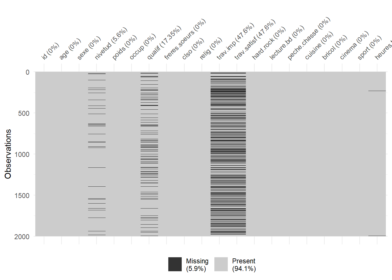
Our dataset contains 9.9% of missings values, and those missings mostly come from trav.imp (47.6%), trav.satisf (47.6%), qulif (17.4%) and nivetud (5.6%).
naniar has other useful functions to handle missing data, such as n_var_miss() which gives you the number of variables containing missing values.
Sometimes we want to see the statistics broken down by a categorical variable. For that, we can use the powerful functions from dplyr packages, which comes with tidyverse.
hdv2003 %>%
  group_by(trav.satisf) %>%
  summarise(min    = min(heures.tv, na.rm = T),
            mean   = mean(heures.tv, na.rm = T),
            median = median(heures.tv, na.rm = T),
            max    = max(heures.tv, na.rm = T))
# A tibble: 4 x 5
  trav.satisf      min  mean median   max
  <fct>          <dbl> <dbl>  <dbl> <dbl>
1 Satisfaction       0  1.62      2     7
2 Insatisfaction     0  2.05      2     6
3 Equilibre          0  1.98      2    10
4 <NA>               0  2.71      3    12
Histograms can help to identify the shape of the distribution of a variable.
ggplot(data = hdv2003) +
  geom_histogram(aes(x = hdv2003$age))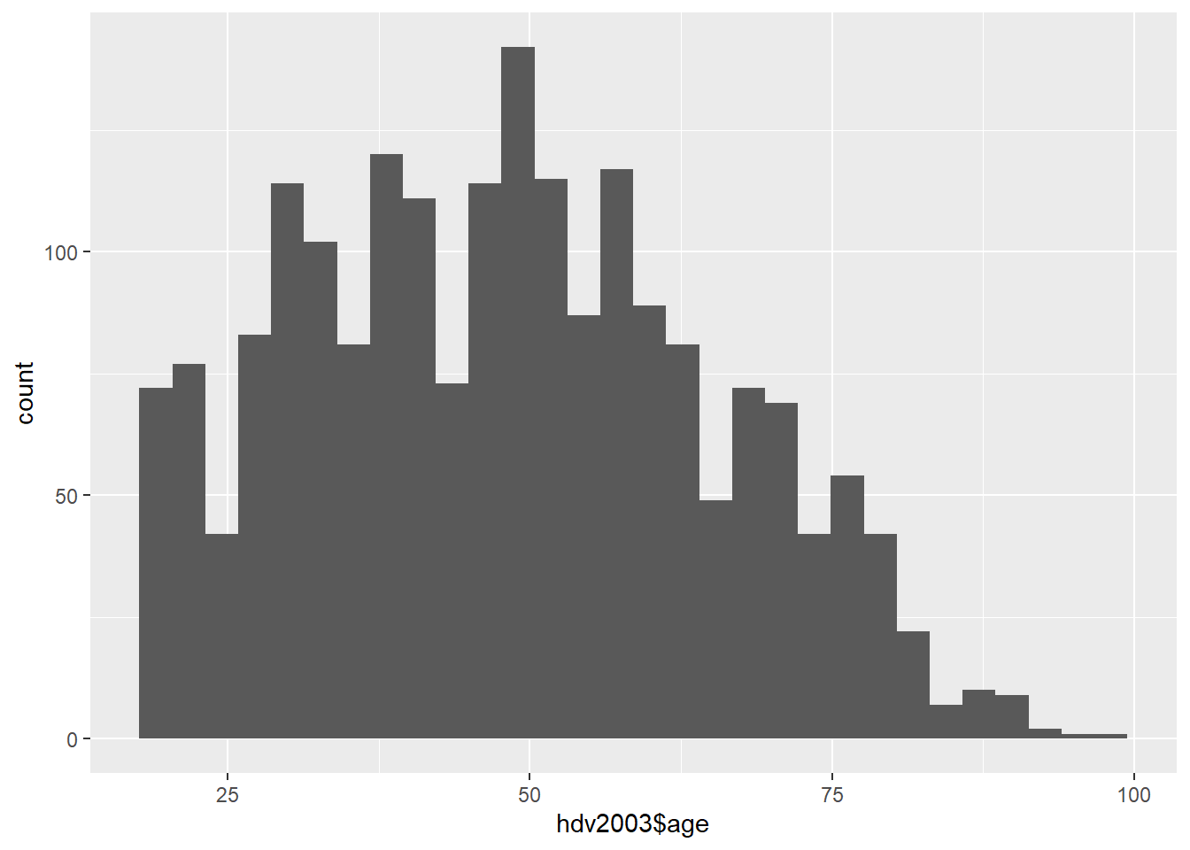
We can see that values are around 50 years and the presence of small queue in the right side.
ggplot2 allows to facet a plot with a categorical variable. To facet with religion, we add facet_wrap(~ relig) to the previous plot.
ggplot(data = hdv2003) +
  geom_histogram(aes(x = hdv2003$age)) +
  facet_wrap(~ relig)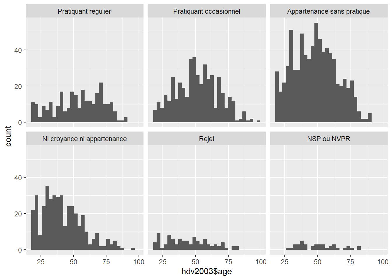
Boxplots can also help to study the distribution, but also for identify outliers (very small or big values).
ggplot(data = hdv2003) +
  geom_boxplot(aes(x = occup, y = heures.tv, color = occup)) +
  theme(legend.position = "none")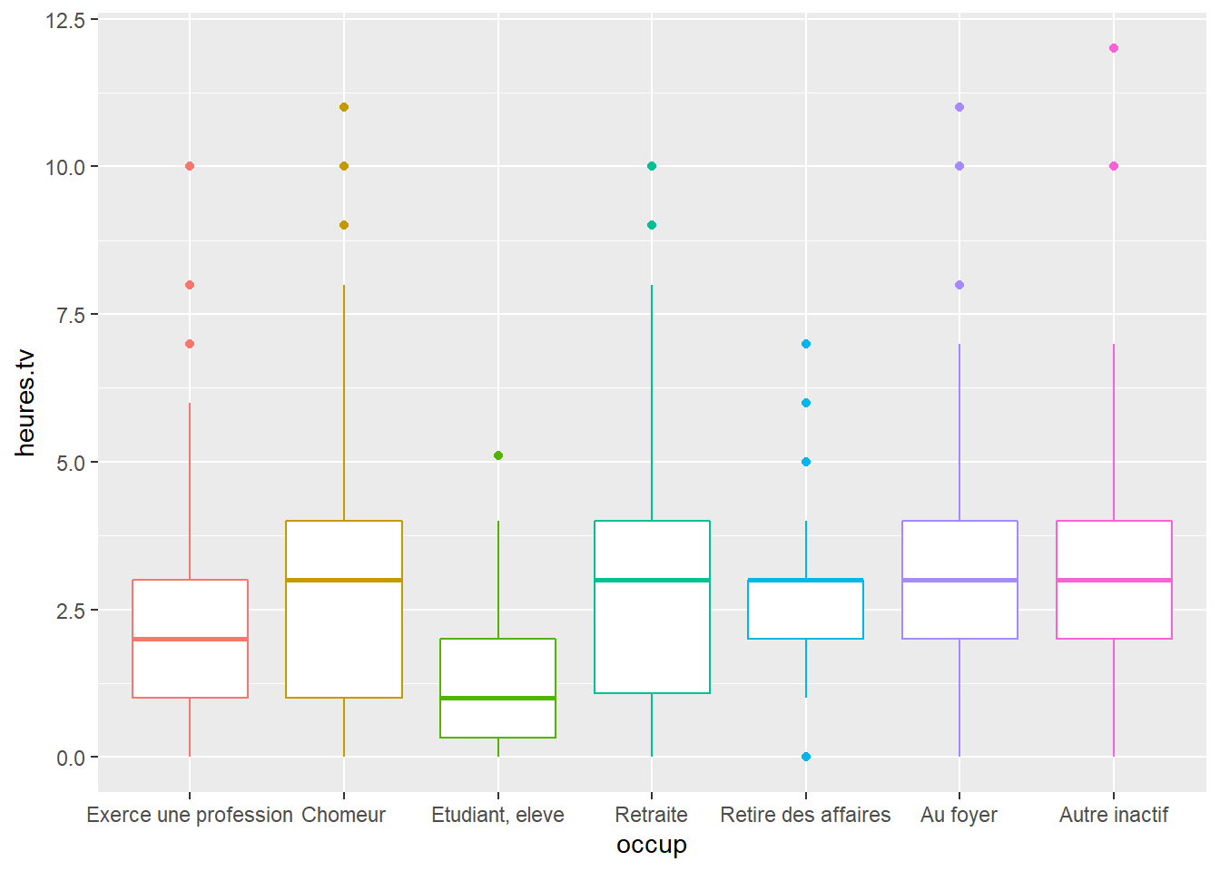
We can also check for relationships among numeric variables using scatterplots.
ggplot(data = hdv2003) +
geom_point(aes(x = age, y = poids, color = sexe)) 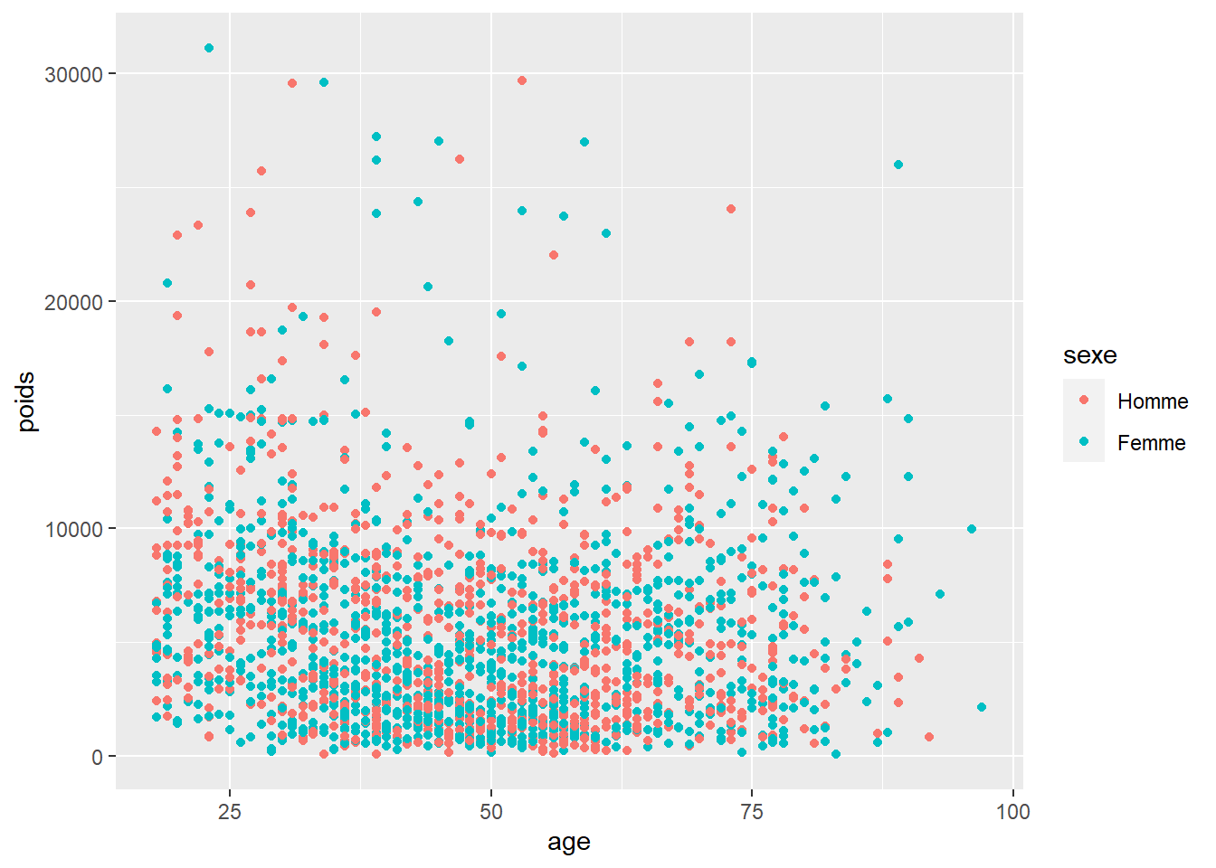
Exploratory Data Analysis can also suggest to recode some variables and or make transformations…
Here we create a new variable minutes.tv which gives the time of watching tv in minutes, using mutate().
hdv2003 %>%
  mutate(minutes.tv = heures.tv * 60) %>%
  select(heures.tv, minutes.tv)
# A tibble: 2,000 x 2
   heures.tv minutes.tv
       <dbl>      <dbl>
 1       0            0
 2       1           60
 3       0            0
 4       2          120
 5       3          180
 6       2          120
 7       2.9        174
 8       1           60
 9       2          120
10       2          120
# ... with 1,990 more rows
Finishing…
We have seen how to perform EDA using some functions of the R language. Summaries, tables and graphics were used to describe data. Results from an Exploratory Data Analysis can help to further with Inferential analysis. For instance, we can test if there is a statistical difference in the time of watching TV among different occupation (occup) categories.
For more reading, check the following links :
All the code of this article and others can be downloaded in Github.
Was this article helpful ? Don’t forget to share it !
TO KUTANI MBALA YA SIMA :)